Some modest insights into the error surface of Neural Nets

Did you know that feedforward Neural Nets (with piecewise linear transfer functions) have no smooth local maxima?

In our recent ICML paper Practical Gauss-Newton Optimisation for Deep Learning) we discuss a second order method that can be applied successfully to accelerate training of Neural Networks. However, here I want to discuss some of the fairly straightforward, but perhaps interesting, insights into the geometry of the error surface that that work gives.

$\newcommand{\br}[1]{\left(#1\right)}$ $\newcommand{\sq}[1]{\left[#1\right]}$ $\newcommand{\ave}[1]{\mathbb{E}\sq{#1}}$

Feedforward Neural Networks

In our description, a feedforward NN takes an input vector $x$ and produces a vector $h_L$ on the final $L^{th}$ layer. We write $h_\lambda$ to be the vector of pre-activation values for layer $\lambda$ and $a_\lambda$ to denote the vector of activation values after passing through the transfer function $f_\lambda$.

Starting with setting $a_0$ to the input $x$, a feedforward NN is defined by the recursion

$$h_\lambda = W_\lambda a_{\lambda-1}$$

where $W_\lambda$ is the weight matrix of layer $\lambda$ (we use a sub or superscript $\lambda$ wherever most convenient) and the activation vector is given by

$$a_\lambda = f_\lambda(h_\lambda)$$

We define a loss $E(h_L,y)$ between the final output layer $h_L$ and a desired training output $y$. For example, we might use a squared loss

$$E(h_L,y) = (h_L-y)^2$$

where the loss is summed over all elements of the vector. For a training dataset the total error function is the summed loss over individual training points

$$\bar{E}(\theta) = \sum_{n=1}^N E(h_L(n),y(n))$$

where $\theta$ represents the stacked vector of all parameters of the network. For simplicity we will write $E(\theta)$ for the error for a single generic datapoint.

The Gradient

For training a NN, a key quantity is the gradient of the error

$$g_{i} = \frac{\partial}{\partial\theta_i} E(\theta)$$

We use this for example in gradient descent training algorithms. An important issue is how to compute the gradient efficiently. Thanks to the layered structure of the network, it’s intuitive that there is an efficient scheme (backprop which is a special case of Reverse Mode AutoDiff) that propagates information from layer to layer.

The Hessian

One aspect of the structure of the error surface is the local curvature, defined by the Hessian matrix with elements

$$H_{ij} = \frac{\partial^2}{\partial\theta_i\partial\theta_j} E(\theta)$$

The Hessian matrix itself is typically very large. To make this more manageable, we’ll focus here on the Hessian of the parameters of a given layer $\lambda$. That is

$$[H_\lambda]_{(a,b),(c,d)} = \frac{\partial^2 E}{\partial W^\lambda_{a,b}\partial W^\lambda_{c,d}}$$

The Hessians $H_\lambda$ then form the diagonal block matrices of the full Hessian $H$.

A recursion for the Hessian

Similar to the gradient, it’s perhaps intuitive that a recursion exists to calculate this layerwise Hessian. Starting from

$$\frac{\partial E}{\partial W^\lambda_{a,b}}=\sum_i \frac{\partial h^\lambda_i}{W^\lambda_{a,b}}\frac{\partial E}{\partial h^\lambda_i} = a^{\lambda-1}_b\frac{\partial E}{\partial h^\lambda_a}$$

and differentiating again we obtain

$$[H_\lambda]_{(a,b),(c,d)} = a^{\lambda-1}_b a^{\lambda-1}_d [{\cal{H}}_\lambda]_{a,c} \tag{1}\label{eq:H}$$

where we define the pre-activation Hessian for layer $\lambda$ as

$$[{\cal{H}}_\lambda]_{a,c} = \frac{\partial^2 E}{\partial h^\lambda_a\partial h^\lambda_c}$$

We show in Practical Gauss-Newton Optimisation for Deep Learning that one can derive a simple backwards recursion for this pre-activation Hessian (the recursion is for a single datapoint – the total Hessian $\bar{H}$ is a sum over the individual datapoint Hessians):

$${\cal{H}}_\lambda = B_\lambda W_{\lambda+1}^\top {\cal{H}}_{\lambda+1}W_{\lambda+1}B_{\lambda}+D_\lambda \tag{2}\label{eq:recursion}$$

where we define the diagonal matrices

$$B_\lambda = \text{diag}(f'_\lambda(h_\lambda))$$

and

$$D_\lambda = \text{diag}\br{f''_\lambda(h_\lambda)\frac{\partial E}{\partial a_\lambda}}$$

Here $f'$ is the first derivative of the transfer function and $f''$ is the second derivative.

The recursion is initialised with ${\cal{H}}_L$ which depends on the objective $E(h_L,y)$ and is easily calculated for the usual loss functions. For example, for the square loss $(y-h_L)^2/2$ we have ${\cal{H}}_L=I$, namely the identity matrix. We use this recursion in our paper to build an approximate Gauss-Newton optimisation method.

Consequences

Piecewise linear transfer functions, such as the ReLU $f(x) = \max(x,0)$ are currently popular due to both their speed of evaluation (compared to more traditional transfer functions such as $\tanh(x)$) and also the empirical observation that, under gradient based training, they tend to get trapped less often in local optima. Note that if the transfer functions are piecewise linear, this does not necessarily mean that the objective will be piecewise linear (since the loss is usually itself not piecewise linear).

For a piecewise linear transfer function, apart from the `nodes’ where the linear sections meet, the function is differentiable and has zero second derivative, $f''(x)=0$. This means that the matrices $D_\lambda$ in the above Hessian recursion will be zero (away from nodes).

For many common loss functions, such as squared loss (for regression) and cross entropy loss (for classification) the Hessian ${\cal{H}}_L$ is Positive Semi-Definite (PSD).

Note that, according to \eqref{eq:recursion}, for transfer functions that contain zero gradient points $f'(x)=0$ then the Hessian $H_\lambda$ can have lower rank than $H_{\lambda+1}$, reducing the curvature information propagating back from layers close to the output towards layers closer to the input. This has the effect of creating flat plateaus in the surface and makes gradient based training potentially more problematic. Conversely, provided the gradient of the transfer function is never zero $f'\neq 0$, then according to \eqref{eq:recursion} each layer pre-activation Hessian is Positive Definite, helping preserve the propagation of surface curvature back through the network.

Structure within a layer

For such loss functions, it follows that the pre-activation Hessian ${\cal{H}}_\lambda$ for all layers is PSD as well (away from nodes). It immediately follows from \eqref{eq:H} that the Hessian $H_\lambda$ for each layer $\lambda$ is PSD. This means that, if we fix all the parameters of the network, and vary only the parameters in a layer $W^\lambda$, then the objective $E$ can exhibit no smooth local maxima or smooth saddle points. Note that this does not imply that the objective is convex everywhere with respect to $W_\lambda$ as the surface will contain ridges corresponding to the non-differentiable nodes.

No differentiable local maxima

The trace of the full Hessian $H$ is the sum of the traces of each of the layerwise blocks $H_\lambda$. Since (as usual away from nodes) by the above argument each matrix $H_\lambda$ is PSD, it follows that the trace of the full Hessian is non-negative. This means that it is not possible for all eigenvalues of the Hessian to be simultaneously negative, with the immediate consequence that feedforward networks (with piecewise linear transfer functions) have no differentiable local maxima. The picture below illustrates the kind of situtation therefore that can happen in terms of local maxima:

whereas the image below depicts the kind of smooth local maxima that cannot happen:

Visualisation for a simple two layer net

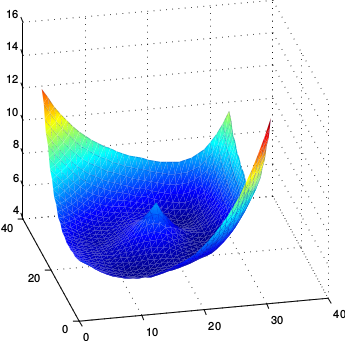
We consider a simple network with two layers, ReLU transfer functions and square loss error. The network thus has two weight matrices $W^1$ and $W^2$. Below we choose two fixed matrices $U$ and $V$ and parameterise the weight matrix $W^1$ as a function of two scalars $u$ and $v$, so that $W^1(u,v)=uU + vV$. As we vary $u$ and $v$ we then plot the objective function $E(u,v)$, keeping all other parameters of the network fixed.

As we can see the surface contains no local differentiable local maxima as we vary the parameters in the layer.

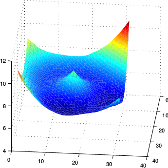
Below we show an analogous plot for varying the parameters of the second layer weights $W^2(u,v)$, which has the same predicted property that there are no differentiable local maxima.

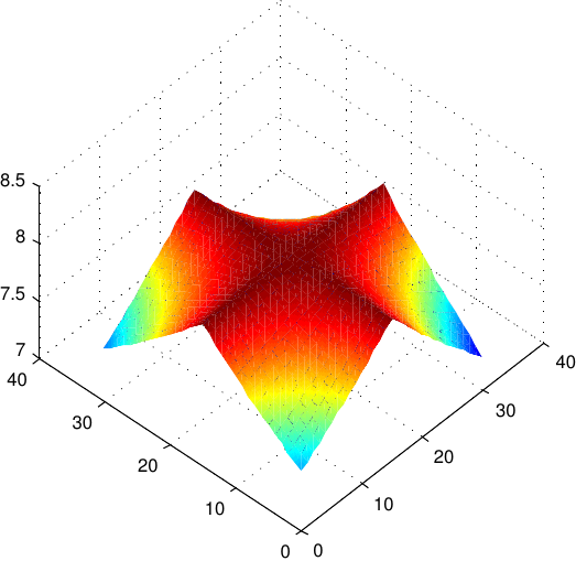
Finally, below we plot $E(u,v)$ using $W^1=uU$ and $W^2=vV$, showing how the objective function changes as we simultaneously change the parameters in different layers. As we can see, there are no differentiable maxima.

Summary

A simple consequence of using piecewise linear transfer functions and a convex loss, is that feedforward networks cannot have any differentiable maxima (or saddle points) as parameters are varied within a layer. Furthermore, the objective cannot contain any differentiable maxima, even as we vary parameters across layers. Note that the objective $E(u,v)$ though can (and empirically does) have smooth saddle points as one varies parameters $u$ and $v$ across different layers.

It’s unclear how practically significant these modest insights are. However, they do potentially partially support the use of piecewise linear transfer functions (particularly those with no zero gradient regions) since for such transfer functions gradient based training algorithms cannot easily dawdle on local maxima (anywhere), or idle around saddle points (within a layer) since such regions correspond to sharp slopes in the objective.

These results are part of a more detailed study of second order methods for optimisation in feedforward Neural Nets which will appear in ICML 2017.