Evolutionary Optimization as a Variational Method

How popular evolutionary style optimisation methods can be viewed as optimisation of a rigorous bound.

$\newcommand{\sq}[1]{\left[#1\right]}$ $\newcommand{\ave}[1]{\mathbb{E}\sq{#1}}$

Variational Optimization is based on the bound

$$min_x f(x) \leq \ave{f(x)}_{p(x|\theta)}$$

That is, the minimum of a collection of values is always less than their average. By defining

$$U(\theta) = \ave{f(x)}_{p(x|\theta)}$$

instead of minimising $f$ with respect to $x$, we can minimise the upper bound $U$ with respect to $\theta$. Provided the distribution $p(x\vert \theta)$ is rich enough, this will be equivalent to minimising $f(x)$.

The gradient of the upper bound is then given by

$$\frac{\partial U}{\partial \theta} = \ave{f(x)\frac{\partial}{\partial \theta}\log p(x|\theta)}_{p(x|\theta)}$$

which is reminiscent of the REINFORCE (Williams 1992) policy gradient approach in Reinforcement Learning.

In the original VO report and paper this idea was used to form a differentiable upper bound for non-differentiable $f$ and also discrete $x$.

Sampling Approximation

There is an interesting connection to evolutionary computation (more precisely Estimation of Distribution Algorithms) if the expectation with respect to $p(x\vert \theta)$ is performed using sampling. In this case one can draw samples $x^1,\ldots,x^S$ from $p(x\vert\theta)$ and form an unbiased approximation to the upper bound gradient

$$\frac{\partial U}{\partial \theta} \approx \frac{1}{S} \sum_{s}f(x^s)\frac{\partial}{\partial \theta}\log p(x^s|\theta)$$

The “evolutionary” connection is that the samples $x^s$ can be thought of as “particles” or “swarm members” that are used to estimate the gradient. Based on the approximate gradient, simple Stochastic Gradient Descent (SGD) would then perform the parameter update (for learning rate $\eta$)

$$\theta^{new} = \theta-\frac{\eta}{S} \sum_{s}f(x^s)\frac{\partial}{\partial \theta}\log p(x^s|\theta)$$

The “swarm” then disperses and draws a new set of members from $p(x\vert \theta^{new})$ and the process repeats.

A special case of VO is to use a Gaussian so that (for the scalar case – the multivariate setting follows similarly)

$$U(\theta) = \frac{1}{\sqrt{2\pi\sigma^2}}\int e^{-\frac{1}{2\sigma^2}(x-\theta)^2}f(x)dx$$

Then the gradient of this upper bound is given by

$$U'(\theta) = \frac{1}{\sigma^2}\ave{(x-\theta)f(x)}_{x\sim N(\theta,\sigma^2)}$$

By changing variable $\epsilon=x-\theta$ this is equivalent to

$$U'(\theta) = \frac{1}{\sigma^2}\ave{\epsilon f(\theta+\epsilon)}_{\epsilon \sim N(0,\sigma^2)} \label{eq:grad}\tag{1}$$

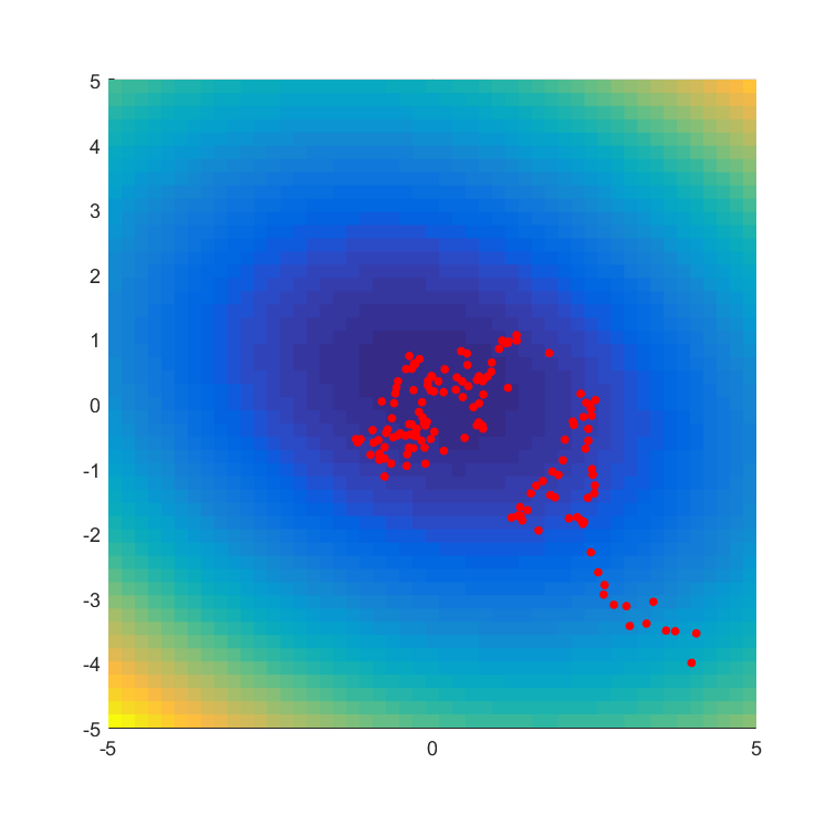
Fixing $\sigma=5$ and using $S=10$ samples, we show below the trajectory (for 150 steps of SGD with fixed learning rate $\eta=0.1$) of $\theta$ based on Stochastic VO and compare this to the underlying function $f(x)$ (which in this case is a simple quadratic). Note that we only plot below the parameter $\theta$ trajectory (each red dot represents a parameter $\theta$, with the initial parameter in the bottom right) and not the samples from $p(x\vert \theta)$. As we see, despite the noisy gradient estimate, the parameter values $\theta$ move toward the minimum of the objective $f(x)$. The matlab code is available if you’d like to play with this.

One can also consider the bound as a function of both the mean $\theta$ and variance $\sigma^2$:

$$U(\theta,\sigma^2) = \frac{1}{\sqrt{2\pi\sigma^2}}\int e^{-\frac{1}{2\sigma^2}(x-\theta)^2}f(x)dx$$

and minimise the bound with respect to both $\theta$ and $\sigma^2$ (which we will parameterise using $\sigma^2=e^\beta$ to ensure a positive variance). More generally, one can consider parameterising the Gaussian covariance matrix for example using factor analysis and minimsing the bound with respect to the factor loadings.

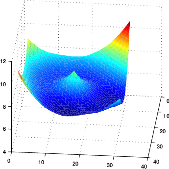
Using a Gaussian with covariance $e^\beta I$ and performing gradient descent on both $\beta$ and $\theta$, for the same objective function, learning rate $\eta=0.1$ and initial $\sigma=5$, we obtain the trajectory below for $\theta$

As we can see, by learning $\sigma$, the trajectory is much less noisy and more quickly homes in on the optimum. The trajectory of the learned standard deviation $\sigma$ is given below, showing how the variance reduces as we home in on the optimum.

In the context of more general optimisation problems (such as in deep learning and reinforcement learning), VO is potentially interesting since the sampling process can be distributed across different machines.

Gradient Approximation by Gaussian Perturbation

Ferenc Huszar‏ has a nice post Evolution Strategies: Almost Embarrassingly Parallel Optimization summarising recent work by Salimans etal on Evolution Strategies as a Scalable Alternative to Reinforcement Learning.

The aim is to minimise a function $f(x)$ by using gradient based approaches, without explicitly calculating the gradient. The first observation is that the gradient can be approximated by considering the Taylor expansion

$$f(x+\epsilon) = f(x)+\epsilon f'(x) + \frac{\epsilon^2}{2} f''(x) + O(\epsilon^3)$$

Multiplying both sides by $\epsilon$

$$\epsilon f(x+\epsilon) = \epsilon f(x)+\epsilon^2 f'(x) +\frac{\epsilon^3}{2}f''(x)+ O(\epsilon^4)$$

Finally, taking the expectation with respect to $\epsilon$ drawn from a Gaussian distribution with zero mean and variance $\sigma^2$ we have

$$\ave{\epsilon f(x+\epsilon)} = \sigma^2 f'(x) + O(\epsilon^4)$$

Hence, we have the approximation

$$f'(x) \approx \frac{1}{\sigma^2}\ave{\epsilon f(x+\epsilon)} \label{eq:grad2}\tag{2}$$

Based on the above discussion of VO, and comparing equations (1) and (2) we see that this Gaussian perturbation approach is related to VO in which we use a Gaussian $p(x\vert \theta)$, with the understanding that in the VO case the optimisation is over $\theta$ rather than $x$. An advantage of the VO approach, however, is that it provides a principled way to adjust parameters such as the variance $\sigma^2$ (based on minimising the upper bound).

Whilst this was derived for the scalar setting, the vector derivative is obtained by applying the same method, where the $\epsilon$ vector is drawn from the zero mean multivariate Gaussian with covariance $\sigma^2 I$ for identity matrix $I$.

Efficient Communication

A key insight in Evolution Strategies as a Scalable Alternative to Reinforcement Learning is that the sampling process can be distributed across multiple machines, $i\in\{1,\ldots,S\}$ so that

$$f'(x) \approx \frac{1}{S\sigma^2}\sum_{i=1}^S {\epsilon^i f(x+\epsilon^i)}$$

where $\epsilon^i$ is a vector sample and $i$ is the sample index. Each machine $i$ can then calculate $f(x+\epsilon^i)$. The Stochastic Gradient parameter update with learning rate $\eta$ is

$$x^{new} = x - \frac{\eta}{S\sigma^2}\sum_{i=1}^S {\epsilon^i f(x+\epsilon^i)}$$

Provided each machine $i$ also knows the random seed used to generate the $\epsilon^j$ of each other machine, it therefore knows what all the $\epsilon^j$ are (by sampling according to the known seeds) and can thus calculate $x^{new}$ based on only the $S$ scalar values calculated by each machine. The basic point here is that, thanks to seed sharing, there is no requirement to send the vectors $\epsilon^i$ between the machines (only the scalar values $f(x+\epsilon^i)$ need be sent), keeping the transmission costs very low.

Based on the insight that the Parallel Gaussian Perturbation approach is a special case of VO, it would be natural to apply VO using seed sharing to efficiently parallelise the sampling. This has the benefit that other parameters such as the variance can also be efficiently communicated, potentially significantly speeding up convergence.

Further Work

In our paper¹ we show that approaches such as Natural Evolution Strategies and Gaussian Perturbation, are special cases of Variational Optimization in which the expectations are approximated by Gaussian sampling. These approaches are of particular interest because they are parallelizable. We calculate the approximate bias and variance of the corresponding gradient estimators and demonstrate that using antithetic sampling or a baseline is crucial to mitigate their problems. We contrast these methods with an alternative parallelizable method, namely Directional Derivatives. We conclude that, for differentiable objectives, using Directional Derivatives is preferable to using Variational Optimization to perform parallel Stochastic Gradient Descent.

References

1. T.Bird, J. Kunze, D. Barber. Stochastic Variational Optimization. arxiv.org/abs/1809.04855, 2018. ↩