Training with a large number of classes

In machine learning we often face the issue of a very large number of classes in a classification problem. This causes a bottleneck in the computation. There’s though a simple and effective way to deal with this.

Probabilistic Classification

In areas like Natural Language Processing (NLP) a common task is to predict the next word in sequence (like in preditictive text on a smartphone or in learning word embeddings). For input $x$ and class label $c$, the probability of predicting class $c$ is

$$p_\theta(c|x) = \frac{u_\theta(c,x)}{Z_\theta(x)}$$

where $u_\theta(c,x)$ is some defined function with parameters $\theta$. For example, $u_\theta(c,x)=\exp(w_c'x)$, where $w_c$ is a parameter vector for class $c$ and $x$ is the vector input. The normalising term is

$$Z_\theta(x) = \sum_{c=1}^C u_\theta(c,x)$$

The task is then to adjust the parameters $\theta$ to maximise the probability of the correct class for each of the training points.

However, if there are $C=100,000$ words in the dictionary, this means calculating the normalisation $Z$ for each datapoint is going to be expensive. There have been a variety of approaches suggested over the years to make computationally efficient approximations, many based on importance sampling.

Why plain Importance Sampling doesn’t work

A standard approach to approximating $Z_\theta(x)$ is to use

$$Z_\theta(x) = \sum_{c=1}^C q(c) \frac{u_\theta(c,x)}{q(c)}$$

where $q$ is an importance distribution over all $C$ classes. We can then form an approximation by sampling from $q$ a small number $S$ of classes to form a sample bag ${\cal{S}}$ and using

$$Z_\theta(x) \approx \tilde{Z}_\theta(x) = \frac{1}{S}\sum_{s\in{\cal{S}}} \frac{u_\theta(s,x)}{q(s)}$$

The problem with this approach is that it results in a potentially catastrophic under-estimate of $Z_\theta(x)$. If the classifier is working well, we want that $u_\theta(c,x)$ is much higher than $u_\theta(d,x)$ for any incorrect class $d$. Hence, unless the importance sample bag ${\cal{S}}$ includes class $c$, then the normalisation approximation will miss this significant mass and the probability approximation

$$\frac{u_\theta(c,x)}{\tilde{Z}_\theta(x)}$$

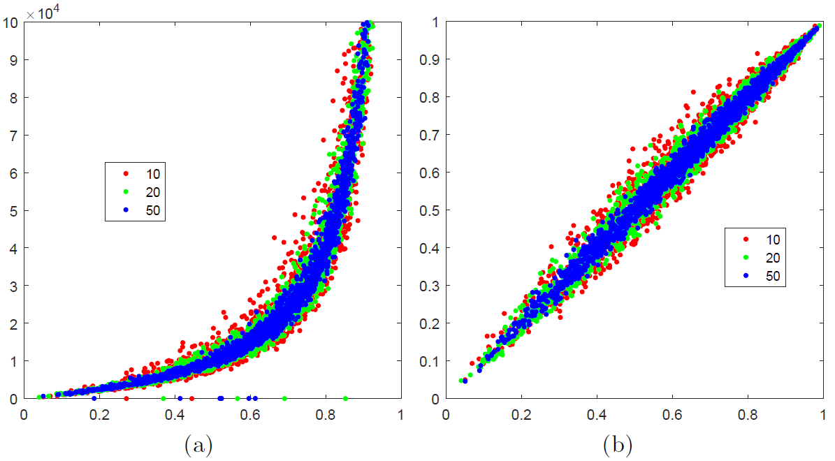
will be wildly inaccurate, see figure (a) below. This is the source of the historically well-documented instabilities in training large-scale classifiers.

Making Importance Sampling work

However, there is an easy fix for this – simply ensure that ${\cal{S}}$ includes the correct class $c$.

On the left above we show for $C=10,000$ classes the ratio $u_\theta(c,x)/Z_\theta(x)$ on the $x$-axis against its approximation $u_\theta(c,x)/\tilde{Z}_\theta(x)$ on the $y$-axis. Each dot represents a different randomly drawn set of $u$ values. Red, green and blue represent 10, 20 and 50 importance samples respectively. The ideal estimation would be such that all points are along the line $y=x$. Note the vertical scale – these values are supposed to be probabilities and lie between 0 and 1. Even as we increase the number of importance samples, this remains a wildly incorrect estimation of the probability.

On the right above we show the same probability estimate but now simply also include the correct class in the set ${\cal{S}}$. The vertical scale is now sensible and the estimated probabiliy is close to the true value.

Deep Learning Recurrent NLP models

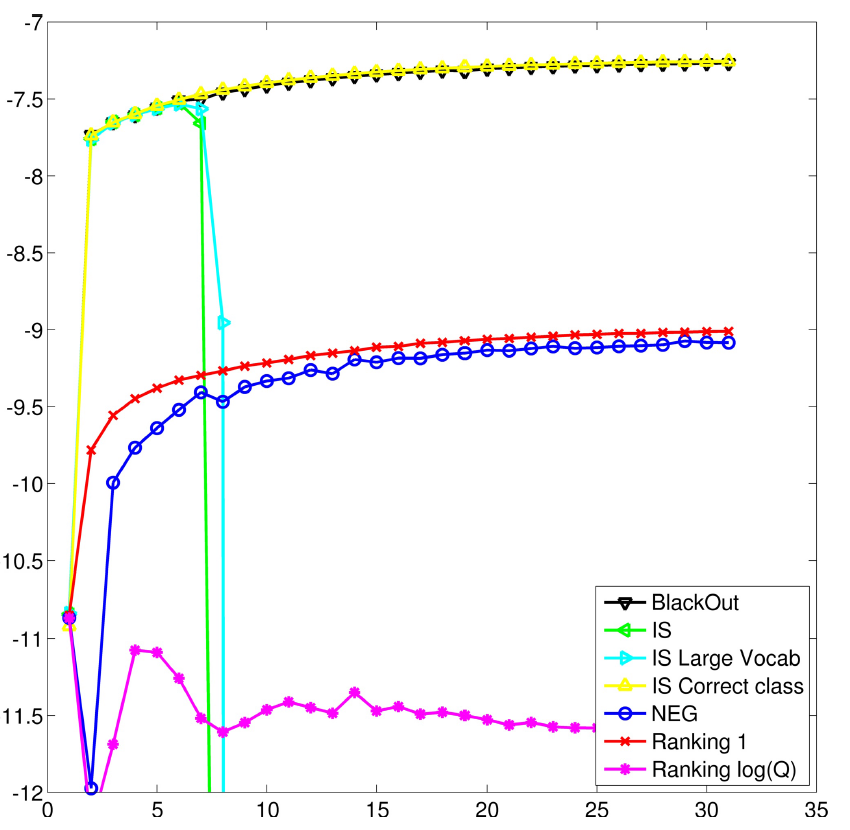
We applied this method to learning word embeddings for a deep recurrent network. The training objective was standard maximum likelihood, but with the normalisation approximation above. Below we plot the exact log likelihood ($y$-axis) against the optimisation gradient ascent iteration ($x$-axis). We also plot the exact log likelihood for some alternative training approaches. As we see, standard Importance Sampling becomes unstable as learning progresses. However our simple modification stabilizes learning and is competitive against a range of alternatives including Noise Contrastive Estimation, Ranking approaches, Negative Sampling and BlackOut.

This is so simple and works so well that we use this in all our NLP deep learning training experiments.

This forms the basis for our paper Complementary Sum Sampling for Likelihood Approximation in Large Scale Classification which will appear in AISTATS 2017.