Training Models that have Zero Likelihood

How can we train generative models when we cannot calculate a gradient likelihood?

A popular class of models in machine learning is the so-called generative model class with deterministic outputs. These are currently used for example in the generation of realistic images. If we represent an image with the variable $x$, then these models generate an image by the following process:

1. Sample $z$ from a $Z$ dimensional Gaussian (multivariate-normal) distribution.

2. Use this $z$ as the input to a deep neural network $g_\theta(z)$ whose output is the image $x$.

Typically the dimension of the latent variable is chosen to be much lower than the observation variable $Z\ll X$. This enables one to learn a low-dimensional representation of high-dimensional observed data.

We can write this mathematically as a latent variable model producing a distribution $p(x)$ over images $x$, with

$$p(x) = \int p(x\vert{}z)p(z)dz$$

and $p(x\vert{}z)$ restricted to a deterministic distribution so that

$$p_\theta(x) = \int \delta\left(x-g_\theta(z)\right)p(z)dz,$$

where we write $p_\theta(x)$ to emphasise that the model depends on the parameters $\theta$ of the network. These models represent a rich class of distributions (thanks to the highly non-linear neural network) and are also easy to sample from (using the above procedure).

So what’s the catch? Given a set of training images, $x^1,\ldots,x^N$, the challenge is to learn the parameters $\theta$ of the network $g_\theta$.

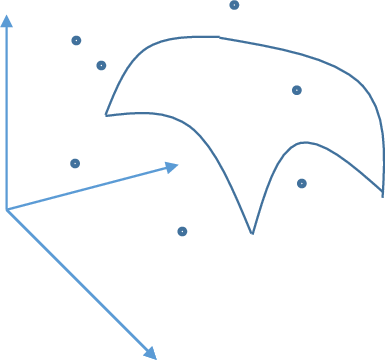
Because the latent dimension $Z$ is lower than the observation dimension $X$, the model can only generate images in a $Z$ dimensional manifold within the $X$ dimensional image space, as depicted in the figure for a latent dimension $Z=2$ and observed dimension $X=3$. That means that only images that lie on this manifold will have non-zero probability density value. For an image $x^n$ from the training dataset, unless it lies exactly on the manifold, the likelihood of this image $p_\theta(x^n)$ will be zero. This means that typically the log likelihood of the dataset

$$L(\theta) \equiv \sum_{n=1}^N \log p_\theta(x^n)$$

is not well defined and standard gradient based training of $L(\theta)$ is not possible. This is a shame because (i) many standard training techniques are based on maximum likelihood and (ii) maximum likelihood is statistically efficient, meaning that no other training method can more accurately learn the model parameters $\theta$.

The inappropriateness of maximum likelihood as the training criterion for this class of models has inspired much recent work. For example the GAN objective and MMD objectives are well known approaches to training such models¹. However, it is interesting to consider whether one can nevertheless modify the maximum likelihood criterion to make it applicable in this situation. The beauty of doing so is that we may then potentially use standard maximum likelihood style techniques (such as variational training approaches).

The Spread Divergence

For concreteness, we consider the Kullback-Leibler Divergence divergence between distributions $p$ and $q$

$$KL(p\vert{}q) \equiv \int p(x)\log \frac{p(x)}{q(x)}dx$$

Maximising the likelihood is equivalent to minimising the KL Divergence between the empirical data distribution

$$p(x)=\frac{1}{N}\sum_{n=1}^N \delta\left(x-x^n\right)$$

and the model $p_\theta(x)$, since

$$KL(p\vert{}p_\theta) = -\frac{1}{N}\sum_{n=1}^N \log p_\theta(x^n) + const$$

The fact that maximum likelihood training is not appropriate for deterministic output generative models is equivalent to the fact that the KL divergence (and its gradient) are not well defined for this class of model.

More generally, for distributions $p$ and $q$, the $f$-Divergence is defined as

$$D_f(p\vert q) = \int f\left( \frac{p(x)}{q(x)}\right) q(x) dx$$

where $f(x)$ is a convex function with $f(1)=0$. However, this divergence may not be defined if the supports (regions of non-zero probability) of $p$ and $q$ are different, since then the ratio $p(x)/q(x)$ can cause a division by zero. This is the situation when trying to define the likelihood for data that is not on the low dimensional manifold of our model.

The central issue we address therefore is how to convert a divergence which is not defined due to support mismatch into a well defined divergence.

From $q(x)$ and $p(x)$ we define new distributions $\tilde{q}(y)$ and $\tilde{p}(y)$ that have the same support. We define distributions

$$\tilde{p}(y) = \int p(y{\mid}x)p(x)dx, \hspace{1cm} \tilde{q}(y) = \int p(y{\mid}x)q(x)dx$$

where $p(y{\mid}x)$ ‘spreads’ the mass of $p$ and $q$ and is chosen such that $\tilde{p}$ and $\tilde{q}$ have the same support.

Consider the extreme case of two delta distributions

$$p(x)=\delta(x-\mu_p), \quad q(x)=\delta(x-\mu_q)$$

for which $KL(p\vert q)$ is not well defined. Using a Gaussian spread distribution $p(y{\mid}x)={\mathcal{N}}(y;x,\sigma^2)$ with mean $x$ and variance $\sigma^2$ ensures that $\tilde{p}$ and $\tilde{q}$ have common support $\mathbb{R}$. Then

$$\tilde{p}(y)=\int \mathcal{N}(y;x,\sigma^2)dx\delta(x-\mu_p)=\mathcal{N}(y;\mu_p,\sigma^2)$$

and

$$\tilde{q}(y)=\int \mathcal{N}(y;x,\sigma^2)dx\delta(x-\mu_q)=\mathcal{N}(y;\mu_q,\sigma^2)$$

and the KL divergence between the two becomes

$$KL(\tilde{p}\vert \tilde{q})=\frac{1}{2\sigma^2}(\mu_p-\mu_q)^2$$

This divergence is well defined for all values of $\mu_p$ and $\mu_q$. Indeed, this divergence has the convenient property that $KL(\tilde{p}\vert \tilde{q})=0 \Rightarrow p=q$. If we consider $p$ to be our data distribution (a single datapoint at $\mu_p$) and $q$ our model $p_\theta$, we can now do a modified version of maximum likelihood training to fit $p_\theta$ to $p$ – instead of minimising $KL(p\vert p_\theta)$, we minimise $KL(\tilde{p}\vert \tilde{p}_\theta)$.

Note that, in general, we must spread both distributions $p$ and $q$ for the divergence between the spreaded distributions to be zero to imply that the original distributions are the same. In the context of maximum likelihood learning, spreading only one of these distributions will in general result in a biased estimator of the underlying model.

Stationary Spread Divergence

If we consider stationary spread distributions of the form $p(y\vert x)=K(y-x)$, for ‘kernel’ function $K(x)$. It is straightforward to show that if the kernel $K(x)$ has strictly positive Fourier Transform, then

$$D_f(\tilde{p}\vert \tilde{q}) = 0 \Rightarrow p=q$$

Interestingly, this condition on the kernel is equivalent to the condition on the kernel in the MMD framework², which is an alternative way to define a divergence between distributions. It is easy to show that the Gaussian distribution has strictly positive Fourier Transform and thus defines a valid spread divergence. Another useful spread distribution with this property is the Laplace distribution.

Machine Learning Applications

We now return to how to train models of the form

$$p_\theta(x) = \int \delta\left(x-g_\theta(z)\right)p(z)dz,$$

and adjust the parameters $\theta$ to make the model fit the data distribution

$$p(x) = \frac{1}{N}\sum_{n=1}^N \delta\left(x-x^n\right)$$

Since maximum likelihood is not (in general) available for this class of models, we instead consider minimising the spread KL divergence using Gaussian spread noise

$$KL(\tilde{p}\vert \tilde{p}_\theta) = -\int \tilde{p}(y) \log \tilde{p}_\theta(y)dy + const$$

where the spreaded data distribution is

$$\tilde{p}(y) = \frac{1}{N}\sum_{n=1}^N \mathcal{N}(y;x^n,\sigma^2 I_X)$$

The objective is then simply an expectation over the log likelihood $\log \tilde{p}_\theta(y)$,

$$\tilde{p}_\theta(y) = \int p(y\vert x)p_\theta(x)dx = \int \mathcal{N}(y; g_\theta(z),\sigma^2 I_X)p(z)dz$$

which is a standard generative model with a Gaussian output distribution. For this we may now use a variational training approach to form a lower bound on the quantity $\log \tilde{p}_\theta(y)$. The final objective just then requires evaluating the expectation of this bound, which can be easily approximated by sampling from the spreaded data distribution.

Overall, this is therefore a simple modification of standard Variational Autoencoder (VAE) training in which there is an additional outer loop sampling from the spreaded data distribution³.

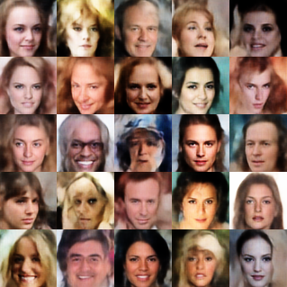
In the figure below we show how we are able to fit a deep generative 4 layer convolutional network with deterministic output to the CelebA dataset of face images. Whilst this model cannot be trained using standard VAE approaches, using the spread divergence approach and sampling from the trained model gives images of the form below

Our aim isn’t to produce the most impressive face sampler, but rather to show how one can make a fairly simple modification of the standard training algorithm to cope with deterministic outputs.

In our paper³ we apply this method to show how to overcome well known problems in training deterministic Independent Components Analysis models using only a simple modification of the standard training algorithm. We also discuss how to learn the spread distribution and how this relates to other approaches such as MMD and GANs.

Summary

A popular class of generative deep network models cannot be trained using standard classical machine learning approaches. However, by adding ‘noise’ to both the model and the data in an appropriate way, one can nevertheless define an appropriate objective that is amenable to standard machine learning training approaches.

References

1. S. Mohamed and B. Lakshminarayanan. Learning in Implicit Generative Models. arxiv.org/abs/1610.03483, 2016. ↩

2. A. Gretton et al. A Kernel Two-Sample Test. Journal of Machine Learning Research, 13. 2012. ↩

3. M. Zhang, P. Hayes, T. Bird, R. Habib, D. Barber. Spread Divergence. arxiv.org/abs/1811.08968, 2018. ↩ ↩²